🤖 Visual Transformer: The Other CNN
ViT Implemented from scratch, explained and demystified 🪄

Hey my friends! Are you interested how those super-smart models "see" and understand images? For years, Convolutional Neural Networks (CNNs) were the undisputed kings of computer vision. But guess what? A new hero is in town, and it's brought a whole new way of thinking: the Visual Transformer (ViT)!
If you're familiar with Transformers in Natural Language Processing (NLP), you know their magic lies in understanding context. ViT essentially takes that same technique and applies it to pixels. Let's break down this fascinating architecture step-by-step, in easy-to-digest manner! (Yummy! 😋)
🔪 Patch Embedder: Slicing a Cucumber
Imagine you have a beautiful image, but a Transformer doesn't "see" pixels like a CNN does. It works with sequences, so our first step is to chop up the image into smaller patches and transform it into "sequence".
The PatchEmbedder class is our kitchen knife for this task.
Instead of traditional slicing and flattening (which can be a bit slow), we use a clever
trick: a 2D convolution layer:
class PatchEmbedder(nn.Module):
    def __init__(self, in_channels, patch_size, hidden_dim):
        super().__init__()
        self.patch_size = patch_size
        self.hidden_dim = hidden_dim

        # we can use classical approach, but conv works faster
        self.patch_embedder = nn.Conv2d(
            in_channels = in_channels,
            out_channels = self.hidden_dim,
            kernel_size = self.patch_size,
            stride = self.patch_size,
        )

    def forward(self, tensor):
        # shape: (bs, hidden_dim = 8, 7, 7)
        conv_embedding = self.patch_embedder(tensor)

        # shape: (bs, 49, hidden_dim = 8)
        embedding = rearrange(conv_embedding, 'b c h w -> b (h w) c')

        return embedding
What's happening here?
nn.Conv2d: This is the star of the show. By settingkernel_sizeandstrideequal to ourpatch_size, the convolution acts like a non-overlapping window. It slides across the image, "seeing" one patch at a time and transforming it into a vector withhidden_dimsize.rearrange(...): After the convolution, our data has a shape like(batch_size, hidden_dim, num_patches_height, num_patches_width). The Transformer prefers a sequence, so we flatten the patch dimensions(h, w)into a single sequence dimension, resulting in(batch_size, num_patches, hidden_dim). For a 28x28 MNIST image with a 4x4 patch size, you get (28/4) * (28/4) = 7 * 7 = 49 patches!
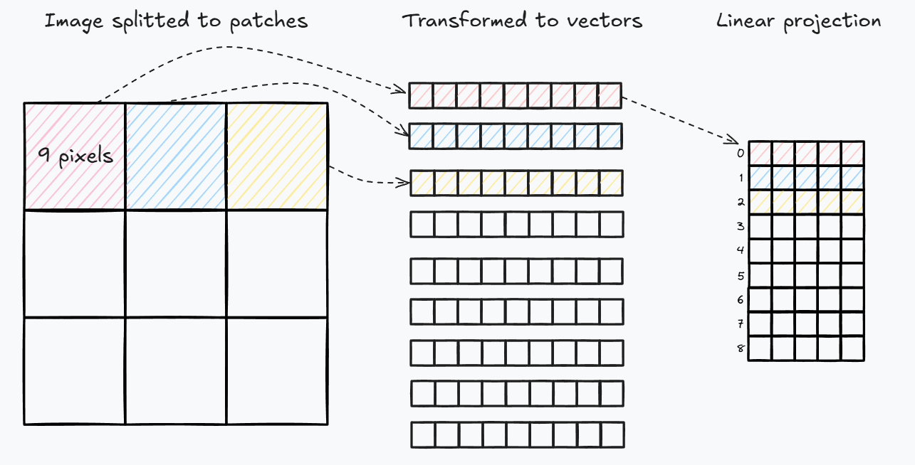
Patch embeddings visualization.
So, we've taken an image and turned it into a sequence of feature vectors, each representing a patch.
THE SHOW STARTS HERE! 🚩
💁 CLS Token and Positional Encoding: Giving Patches Context
Now that we have our sequence of patch embeddings, there are two crucial additions we need to make:
- The CLS (Classification) Token: The CLS token is like a "designated summarizer". It's a special, learnable vector which knows everything about our sequence of patch embeddings. Its job is to accumulate global information from all the patches and eventually be used for classification.
- Positional Encoding: When you read a sentence, the order of words matters. "Dog bites man" is very different from "Man bites dog." Similarly, the spatial position of a patch in an image is crucial. Transformers, by themselves, don't inherently understand order. That's where positional encoding comes in. We add a learnable vector to each patch embedding, unique to its position, so the model knows where each patch belongs in the scheme of the image.
class PositionalEncoder(nn.Module):
    def __init__(self, image_size, patch_size, hidden_dim):
        super().__init__()

        # num_patches = 49 for MNIST
        num_patches = (image_size ** 2) // (patch_size ** 2)

        self.cls_token = torch.nn.Parameter(
            torch.normal(mean=0, std=0.02, size=(1, 1, hidden_dim))
        )

        # shape: (1, 50, 8), all patches and cls token.
        # We do it learnable, but can use sinusod fixed encodings
        self.positional_embeddings = torch.nn.Parameter(
            torch.normal(mean=0, std=0.02, size=(1, num_patches + 1, hidden_dim))
        )

    def forward(self, patch_embeddings):
        cls_token = self.cls_token.expand(patch_embeddings.size(0), -1, -1)
        cls_patch_embeddings = torch.cat((cls_token, patch_embeddings), dim=1)
        return cls_patch_embeddings + self.positional_embeddings
Breaking it down:
self.cls_token: This is our special classification token, initialized randomly and will be learned during training. Weexpandit to match the batch size.torch.cat(...): We concatenate the CLS token with our patch embeddings along the sequence dimension. Now our sequence is(batch_size, num_patches + 1, hidden_dim).self.positional_embeddings: Similar to the CLS token, these are learnable embeddings for each position. We simply add them to our combined (CLS + patch) embeddings. This simple addition is how the model gets its sense of order and location.
At this point, our image is a sequential data stream, complete with spatial context and a global summary token, ready for the Transformer's main event: Attention!
🤯 The Attention Head: "Forgot your head at home, didn't you?"
The core innovation of Transformers is the Self-Attention mechanism. It allows each patch to "look at" every other patch (and the CLS token) in the sequence and decide how important they are to its own understanding.
Each AttentionHead calculates three things for every input vector (patch or
CLS token):
- Query (Q): What am I looking for?
- Key (K): What do I have?
- Value (V): What information do I carry?
class AttentionHead(nn.Module):
    def __init__(self, hidden_dim, head_size):
        super().__init__()

        self.head_size = head_size

        self.wq = nn.Linear(hidden_dim, head_size, bias=False)
        self.wk = nn.Linear(hidden_dim, head_size, bias=False)
        self.wv = nn.Linear(hidden_dim, head_size, bias=False)

    def forward(self, input):
        Q = self.wq(input) # (bs, 50, 4)
        K = self.wk(input)
        V = self.wv(input)

        attention = Q @ K.transpose(-2, -1) # (bs, 50, 50)
        attention = attention / (self.head_size ** 0.5)
        attention = torch.softmax(attention, dim=-1)

        attention = attention @ V # (bs, 50, 4)

        return attention
Here's the formula:
$$ \text{Attention}(Q, K, V) = \text{softmax}\left(\frac{QK^T}{\sqrt{d_k}}\right)V $$
Where \(d_k\) is head_size (the dimension of the keys).
This scaling factor prevents very large values in the dot product from pushing the
softmax into regions with tiny gradients.
A bit more explanation:
- We project our input into Query, Key, and Value representations using linear layers.
- We calculate
attention_scoresby taking the dot product of Query with all Keys (\(QK^T\)). This tells us how well each patch's "query" matches every other patch's "key." A higher score means more relevance. - We divide by the square root of
head_sizefor stabilization. torch.softmaxturns these scores into probabilities (attention_weights), ensuring they sum to 1. This is how each patch decides how much "attention" to give to other patches.- Finally, we multiply these
attention_weightsby the Value vectors (\(attention\_weights \cdot V\)). This means patches that are deemed more relevant contribute more to the output.
The result is a new representation for each patch, enriched with information from all other patches, weighted by their relevance!
🗣️🗣️🗣️ Multi-Head Attention: Many Heads Are Better Than One
"WE NEED TO STACK MORE LAYERS!" - remember?" One attention head is really good, but what if different heads could focus on different aspects of relationships between patches? That's the idea behind Multi-Head Self-Attention (MHSA)!
Instead of just one attention calculation, we run several AttentionHead in
parallel.
Each head learns different Q, K, V projections and therefore captures different types of
relationships.
class AttentionMultiHead(nn.Module):
    def __init__(self, hidden_dim, head_size, num_heads):
        super().__init__()

        self.heads = torch.nn.ModuleList(
            [AttentionHead(hidden_dim, head_size) for _ in range(num_heads)]
        )

        self.dim_restoration = torch.nn.Linear(head_size * num_heads, hidden_dim)

    def forward(self, input):
        """ Result dimensionality is the same as input """
        head_outputs = [head(input) for head in self.heads]
        stacked_heads = torch.cat(head_outputs, dim = -1)
        result = self.dim_restoration(stacked_heads)
        return result
How it works:
- We create a list of independent
AttentionHeadinstances. - In the
forwardpass, each head processes the input independently. - The outputs from all heads are then concatenated (
torch.cat) along the feature dimension. If you havenum_headsheads, each producinghead_sizefeatures, you'll get a concatenated vector of sizehead_size * num_heads. - Finally, a linear layer (
self.dim_restoration) projects this concatenated output back to the originalhidden_dim, ensuring that the input and output dimensionality of the MHSA block remain consistent. This is super important for stacking multiple blocks!
Multi-Head Attention allows the model to simultaneously attend to information from different representation subspaces at different positions. It's literally a team of multiple experts analyzing the same problem from different angles. Junior, middle, senior.. you know 😂
💪 The Transformer Encoder Block: The Core
Now we combine Multi-Head Self-Attention with a few other components to form a complete Transformer Encoder Block. This block is repeated multiple times to build the full Transformer.
class BlockViT(nn.Module):
    def __init__(self, hidden_dim, head_size, num_heads, mlp_hidden_size):
        super().__init__()

        self.norm1 = nn.LayerNorm(hidden_dim)
        self.mhsa = AttentionMultiHead(hidden_dim, head_size, num_heads)
        self.norm2 = nn.LayerNorm(hidden_dim)

        self.mlp = torch.nn.Sequential(
            torch.nn.Linear(hidden_dim, mlp_hidden_size),
            torch.nn.GELU(),
            torch.nn.Linear(mlp_hidden_size, hidden_dim)
        )

    def forward(self, input):
        out = input + self.mhsa(self.norm1(input))
        out = out + self.mlp(self.norm2(out))
        return out
Let's unpack this powerhouse:
nn.LayerNorm(...): Normalization layers are crucial for stable training, especially in deep networks. They normalize the input features across the hidden dimension.self.mhsa(...): Our Multi-Head Self-Attention.self.mlp(...): A simple Feed-Forward Network (Multi-Layer Perceptron) with two linear layers and a GELU activation function in between. This allows the model to process the information learned by attention further.- Residual Connections (
input + ...andout + ...): This is a critical component borrowed from ResNets (We didn't forget you, grandfather 👴). It helps information flow more easily through very deep networks by adding the input directly to the output of a sub-layer. This prevents vanishing gradients and allows for deeper models.
So, each block takes our sequence of embeddings, normalizes it, applies multi-head attention, normalizes it again, applies an MLP, and finally adds back the original input (residual connection) to ensure smooth information flow. This process refines the understanding of each patch's context.
🏁 Assembling the SimpleViT: The Grand Finale!
Finally, let's put all the pieces together into our complete SimpleViT
model!
class SimpleViT(nn.Module):
    def __init__(self, in_channels, image_size, patch_size, hidden_dim, num_layers, head_size, num_heads, mlp_hidden_size):
        super().__init__()

        self.patch_embedder = PatchEmbedder(in_channels, patch_size, hidden_dim)
        self.positional_encoder = PositionalEncoder(image_size, patch_size, hidden_dim)

        self.encoder_blocks = torch.nn.Sequential(
            *[BlockViT(hidden_dim, head_size, num_heads, mlp_hidden_size) for _ in range(num_layers)]
        )

        self.classifier = torch.nn.Sequential(
            torch.nn.Linear(hidden_dim, 10),
            nn.Softmax(dim=-1)
        )


    def forward(self, image):
        patch_embeddings = self.patch_embedder(image)
        positional_encoded_embeddings = self.positional_encoder(patch_embeddings)
        encodings = self.encoder_blocks(positional_encoded_embeddings)

        cls_token = encodings[:, 0, :]
        classification_result = self.classifier(cls_token)

        return classification_result
The full journey of an image through SimpleViT:
- An image first goes through the
patch_embedder, getting chopped into patches and converted into a sequence of feature vectors. - Then, the
positional_encoderadds a special CLS token and positional information to these patch embeddings. - This enriched sequence is then fed through a series of
encoder_blocks(num_layersof them). Each block refines the understanding of the relationships between patches. - After all the encoder blocks, we're left with a highly contextualized sequence.
We're primarily interested in the
cls_token(the first element,encodings[:, 0, :]) because it has absorbed information from all other patches and represents the global context. - Finally, this
cls_tokenis passed through a simpleclassifier(a linear layer followed by Softmax) to predict the class of the input image!
And there you have it! A complete Visual Transformer, built from the ground up.
📌Conclusion: A New Era for Computer Vision?
The Visual Transformer represents a paradigm shift in computer vision. By adapting the incredibly successful Transformer architecture from NLP, ViT has shown that images can be treated as sequences of patches, opening up new directions for how we process visual data. It's often called as the "new CNN" because it achieves state-of-the-art results on many image recognition tasks, often with fewer inductive biases than traditional CNNs.
While CNNs have their strengths, ViT's ability to capture long-range dependencies across an image (thanks to self-attention) makes it incredibly powerful. It's a testament to the power of generalization in AI research, proving that architectures designed for one domain can find huge success in another!
Want to dive deeper and see this implementation in action?
🔗 Check out the full repository here: ViT from Scratch.